Constant-time mutual information for Bayesian experimental design

Motivation

A common applied workflow is: collect data, train a model, then deploy it once it is accurate enough. In Bayesian inference, the model encodes your current state of knowledge (and therefore, uncertainty) given what you have observed so far. During data collection, optimal experiment design (OED) uses that current state to decide which experiment or observation to run next so that uncertainty shrinks as quickly as possible. Done well, this can reduce the amount of data you need to reach a useful level of performance, shorten time-to-decision, and avoid spending resources (or opportunity cost) on uninformative measurements.

OED is especially valuable when the pool of possible observations is much larger than what will ever be used for training (clinical trials, A/B testing, ad experiments, surveys): it can be worth spending real compute to choose informative data rather than selecting blindly, because the opportunity cost of collecting the “wrong” data (and delaying decisions) is often larger than the cost of the selection algorithm.

In typical variants of optimal experiment design, this idea is formalized by scoring candidate designs by expected information gain. A common choice is mutual information (MI): the “best” experiment is the one expected to reduce uncertainty the most about whatever you care about (parameters, predictions, or another derived random variable).

Mutual information can be written as an expected reduction in entropy. For a proposed batch design $\mathcal{D}_{1:k}$ and outcomes $y_{1:k}$, the parameter-learning objective is:

I(\theta; y_{1:k} \mid \mathcal{D}_{1:k}) = H\!\left[p(\theta)\right] - \mathrm{E}_{y_{1:k} \sim p(\cdot \mid \mathcal{D}_{1:k})} \left[H\!\left[p(\theta \mid \mathcal{D}_{1:k}, y_{1:k})\right]\right].

Here $\theta$ denotes the current uncertain state of the model at the moment you score designs (e.g., a current posterior state). Intuitively: start from your current uncertainty, then subtract the expected uncertainty after running the batch and updating the model.

Predictive MI uses the same form, replacing $\theta$ with the predictive quantity of interest.

Small modifications are useful when the relevant notion of “uncertainty” isn’t purely Shannon entropy—for example, using similarity-sensitive entropy to encode which distinctions matter for your downstream goal. See Similarity-Sensitive Entropy: Induced Kernels and Data-Processing Inequalities (arXiv:2601.03064) for a framework that helps clarify whether the uncertainty you care about is parameter uncertainty, predictive uncertainty, or uncertainty in some other derived random variable.

Here $k$ is the batch size. The design $\mathcal{D}_{1:k}$ represents a set of $k$ candidate experiments (design points, treatments, prompts, etc.), and $y_{1:k}$ is the corresponding batch of outcomes you will observe. Before data collection, they are unknown, but depend on your model’s predictive distribution and $\mathcal{D}_{1:k}$.

When you can run multiple experiments, selecting the single best experiment (repeatedly choosing $k{=}1$) can be suboptimal: you want a batch that is informative together, avoiding redundancy and covering the space of uncertainty efficiently.

In principle, you can run this continuously: score designs in real time, collect the next batch, update the model, then re-score after every update.

In practice, routinely computing MI inside a live data pipeline is hard:

Batch combinatorics: if you have $n$ candidate experiments and you choose batches of size $k$, there are $\binom{n}{k}$ possible batches. Even with greedy or heuristic search, you end up calling the MI estimator many times.
$k$-dimensional averaging: the expectation over $y_{1:k}$ is a $k$-dimensional sum/integral. Naive enumeration can scale as $2^k$ for binary outcomes, and straightforward quadrature becomes intractable as $k$ grows.
Posterior refresh + state handoff: many estimators assume posterior samples exist (HMC/MCMC). As new data arrives, you pay an inference cost to refresh the model state, ship samples/state to the MI evaluator, score candidate batches, then repeat.
Engineering friction: implementing, tuning, and serving MI under latency constraints doesn’t fit many teams.

Best-first adaptive partitioning

Best-first adaptive partitioning addresses these bottlenecks directly. It's a tree-based adaptive quadrature over the discrete outcome space that performs Bayesian updating inside the MI computation—so you can score candidate batches without maintaining posterior samples or a separate inference service. By using an explicit global refinement budget, per-query compute stays approximately flat as batch size $k$ grows, making it practical to evaluate MI repeatedly in a live design loop.

“Constant-time in $k$” here means: with a fixed global refinement budget, runtime per MI query is approximately independent of $k$. Increasing the budget trades runtime for fidelity.

In integration terms, you can treat it as a single scoring function: given your regression model specification, observed data, and a candidate batch $\mathcal{D}_{1:k}$, it returns an information-gain score for that batch. “Model specification” can be as simple as a likelihood (and, when available, gradients/Hessians for efficient local updates).

information_gain(model_spec, observed_data, candidate_batch) -> score

Where this estimator shines: repeated MI evaluations inside a design loop (especially batch search), where you need a reliable per-query latency budget and don’t want to maintain posterior samples or a separate inference service, or you don't have an inference service at all yet (it comes for free). If you have a highly complex or non-Bayesian model but want to experiment with scoring designs, this can also be a low-overhead way to get started.

Where it’s less compelling: settings where you already have high-quality posterior draws on hand, have highly complex models without analytic likelihoods, or are not bottlenecked by latency.

Integration view: before (two-service pipeline) vs after (single scoring call).

Before · Inference Service

observed_data += new_observations
posterior_samples = run_inference(model_spec, observed_data)   # e.g., HMC/MCMC
artifact_uri = write_to_storage(posterior_samples)             # serialize + publish state

Before · MI Scoring Service

posterior_samples = read_from_storage(artifact_uri)
score = mi_estimate(posterior_samples, candidate_batch)        # repeated many times during batch search

After · Single Scoring Call

observed_data += new_observations
score = information_gain(model_spec, observed_data, candidate_batch)

No posterior samples and no separate inference/scoring service to maintain—just raw data in and an interpretable score out. Dependencies can be minimal: standard numerical linear algebra plus your likelihood/model code.

Results

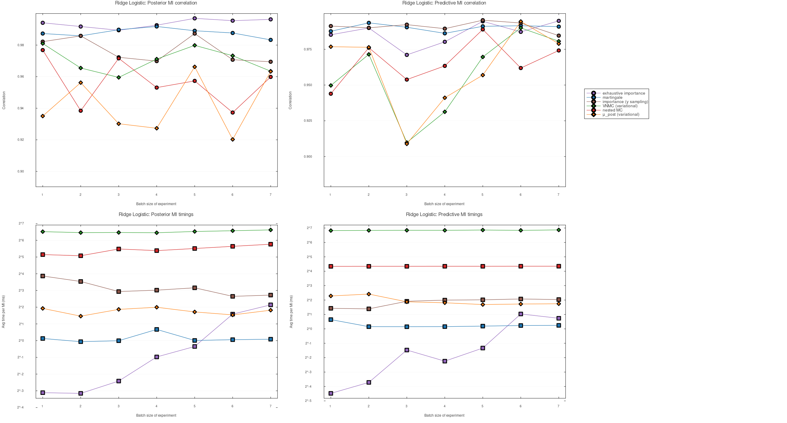
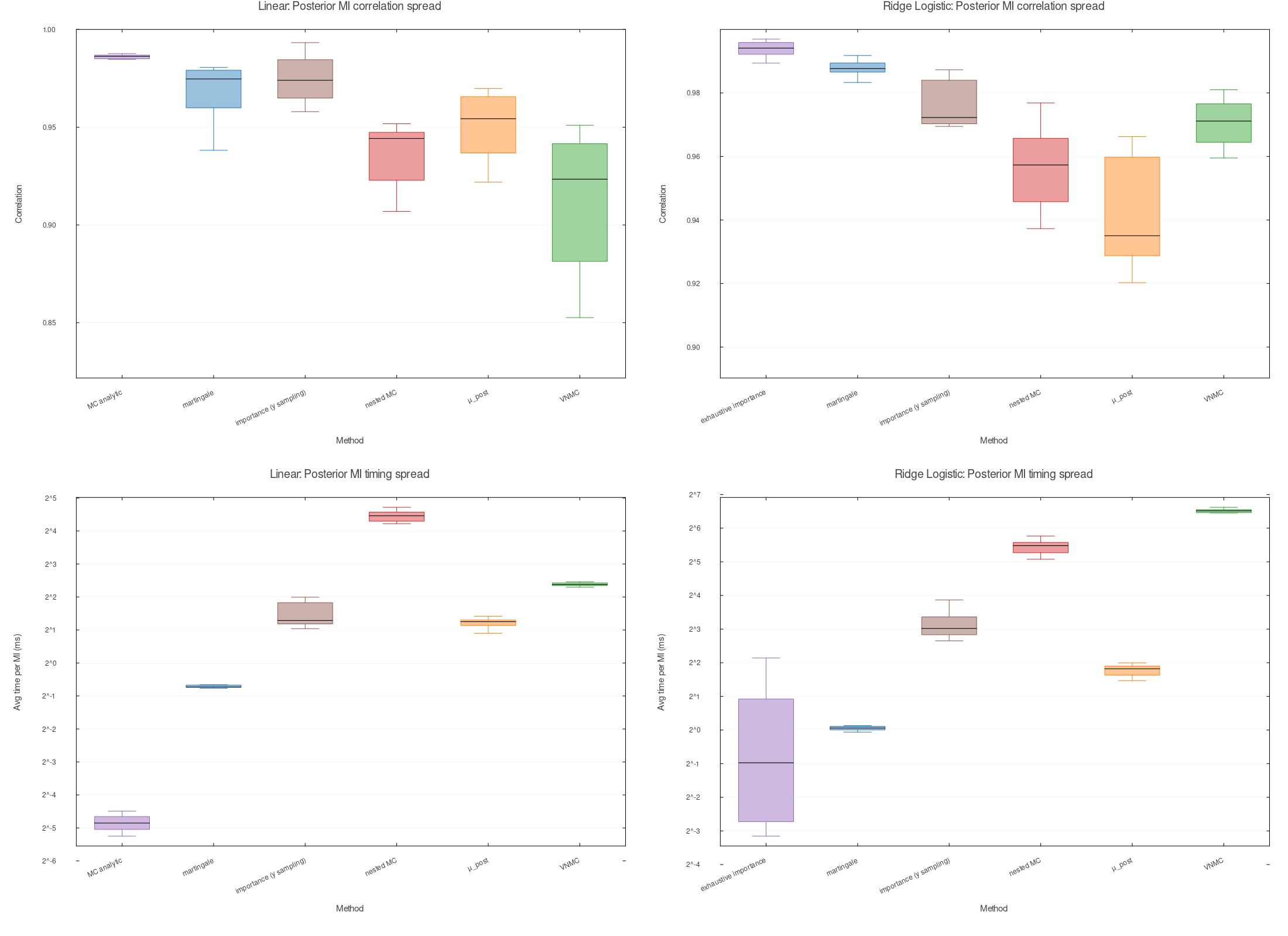
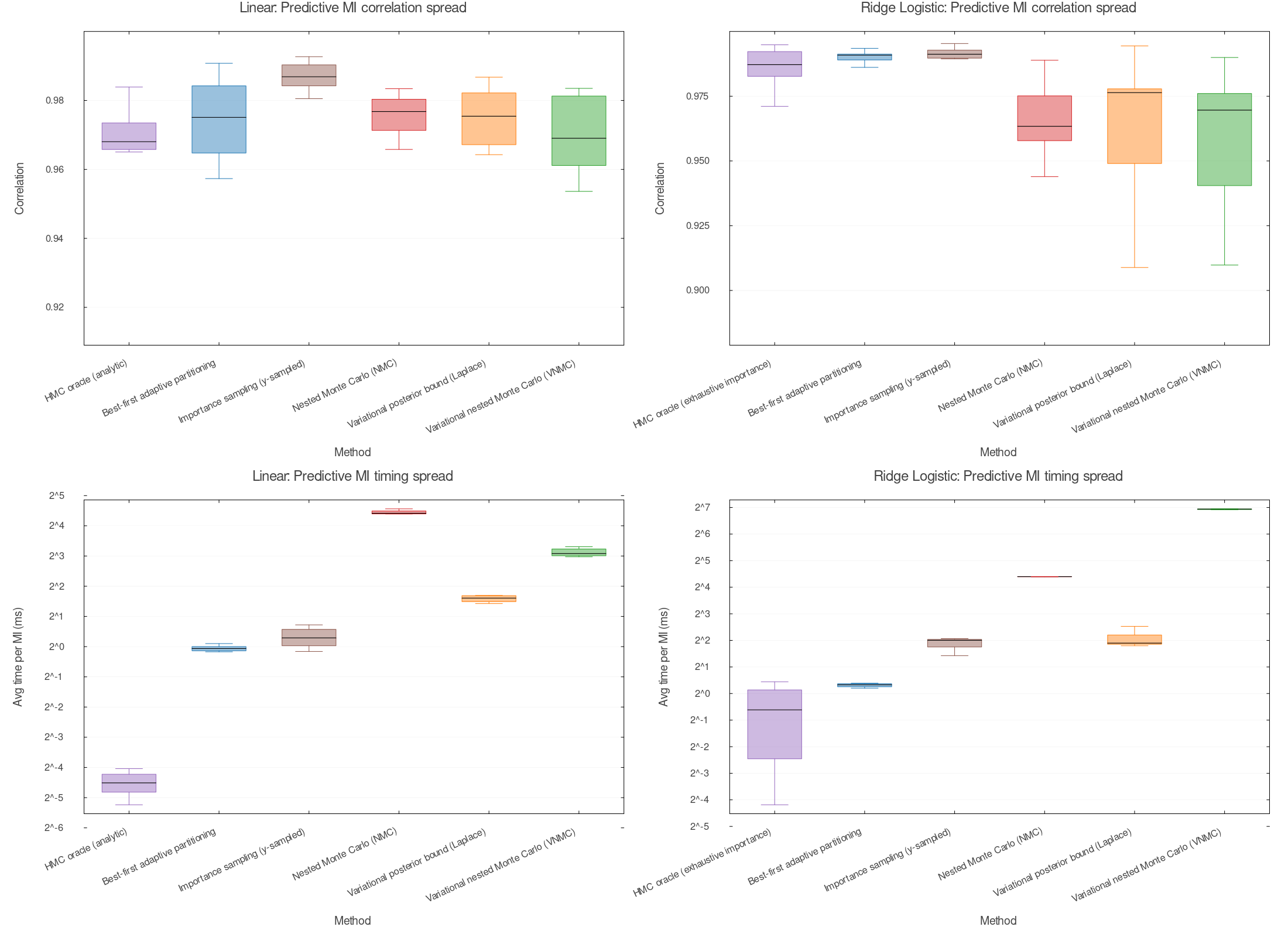
These figures compare multiple estimators of mutual information (MI) used for Bayesian experimental design, across two representative model families (a linear-Gaussian baseline and a nonconjugate ridge-logistic model). The headline: best-first adaptive partitioning delivers an anytime, tunable, constant-time-in-$k$ MI estimator that does not require posterior samples, while remaining competitive in fidelity with strong sampling-based baselines.

For context: on these small benchmarks, refreshing the sampling-based baselines via HMC/MCMC takes about 0.1s (~100ms) per inference run.

Terminology: “Oracle” refers to the high-quality reference used to score fidelity (correlation). In addition, the figures include a couple of problem-specific ceiling baselines (“MC analytic” in the linear-Gaussian case and “Exhaustive importance” in the ridge-logistic case). These are not general-purpose estimators—many models don’t admit shortcuts like these—and they are included to show what’s achievable when you’re willing to write custom, model-tailored machinery for these convenient model classes.

Linear-Gaussian results: correlation and runtime versus batch size k for posterior MI and predictive MI. — **Linear-Gaussian model.** Top row: correlation with the Oracle reference vs batch size $k$ for posterior MI (left) and predictive MI (right). Bottom row: average time per MI query vs $k$. With a fixed refinement budget, best-first adaptive partitioning keeps runtime essentially flat as $k$ grows while maintaining strong correlation.

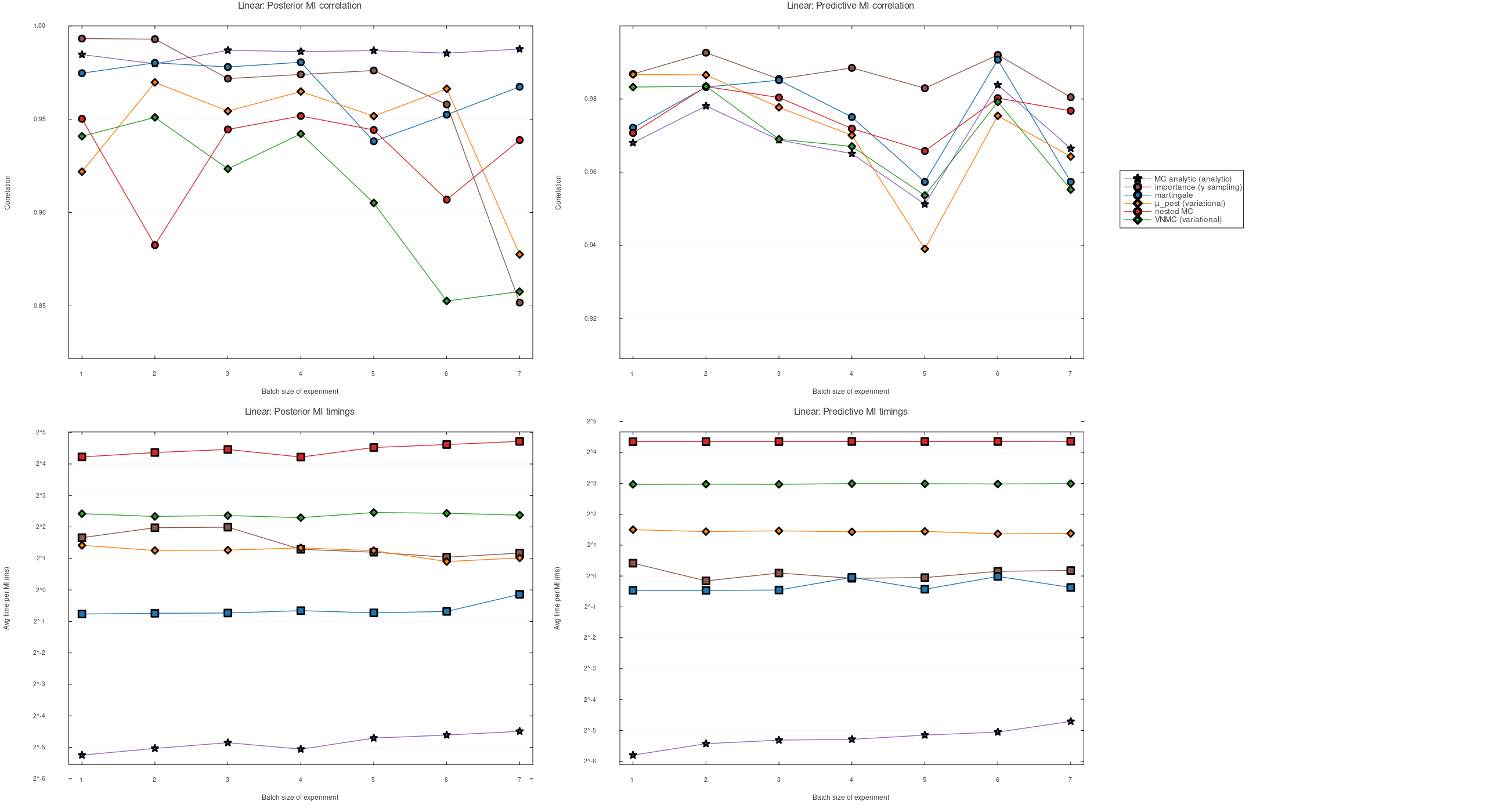
Takeaway: you can hold a strict per-query budget fixed as $k$ grows without giving up strong ranking fidelity.

Ridge-logistic results: correlation and runtime versus batch size k for posterior MI and predictive MI. — **Ridge-logistic model.** The same story holds in a nonconjugate setting: competitive fidelity without posterior samples, and predictable compute thanks to explicit global refinement budgets.

Posterior-MI spread summary: box and whisker plots summarizing variability across batch sizes k for correlation and runtime. — **Across-$k$ variability (posterior MI).** Box/whisker summaries for correlation and time highlight stability and predictable compute for all of the batch sizes tested.

Predictive-MI spread summary: box and whisker plots summarizing variability across batch sizes k for correlation and runtime. — **Across-$k$ variability (predictive MI).** The same spread summaries for the predictive-MI objective.

Evaluation

For each model, we estimate MI for batches of experiments of size $k$, averaged over many randomly chosen design subsets (apples-to-apples across methods at each $k$).
Fidelity (correlation): Pearson correlation across 20 candidate batches between a method’s MI estimates and the Oracle MI values (higher means better MI-based ranking).
Two objectives: posterior MI (learning parameters) and predictive MI (learning predictions at target inputs).
Timing reports average time per MI evaluation (given whatever cached data the method uses), which is the relevant cost when selecting designs by evaluating MI many times.

Comparison protocol:

Sampling-based baselines typically require posterior samples (e.g., via HMC/MCMC). That inference can be a large (though one-time) fixed-data cost, and a practical barrier in real workflows. Best-first adaptive partitioning avoids that dependency by updating posterior state as part of MI estimation.
On these benchmarks the HMC/MCMC inference step is about 0.1s (~100ms), even though the models are small. My estimator takes about 1ms for inference and MI estimation.
To avoid subtle “training on the test set” effects, each sampling-based method uses its own independent posterior draw stream (not shared across methods or with the Oracle reference).

Key takeaways

Predictable compute: fixed refinement budgets keep per-query runtime approximately flat as batch size $k$ grows.
Anytime: usable early scores that improve monotonically as you spend more budget.
Global refinement: spends compute on high-impact outcome regions.
No posterior sampling: Bayesian updating happens inside the MI estimator.
Unified objectives: the same machinery supports posterior and predictive MI.
Drop-in scorer: raw data + candidate batch in, information-gain score out.

MI Algorithms

Best-first adaptive partitioning

Tree-based adaptive quadrature over a discretized outcome space. It starts with a coarse partition, maintains an approximate posterior state per region, and repeatedly refines the regions with the highest estimated global impact—subject to a strict compute budget. Tunable compute via a global refinement budget; no posterior samples required.

From an integration perspective, it can be exposed as a single scoring function from (model spec, observed data, candidate batch) to information gain. The refinement budget is the knob: you trade runtime for fidelity, and you can keep a strict per-query latency target as $k$ grows.

Nested Monte Carlo (NMC)

General-purpose MI estimator with nested sampling loops. Broadly applicable but can be expensive and variance-limited unless inner sample sizes grow.

Variational nested Monte Carlo (VNMC)

Uses variational approximations to tighten bounds and reduce variance relative to NMC, but remains sample-based and still relies on inference machinery.

Variational posterior bound (Laplace)

Fast approximation via a bound and local posterior geometry; performance depends on how well the approximation matches the true posterior (often weaker in nonconjugate regimes).

Importance sampling (y-sampled)

Avoids exhaustive outcome enumeration by sampling outcomes with a proposal distribution; can be brittle when outcomes are imbalanced or proposals mismatch the predictive distribution.

Problem-specific ceiling baselines (MC analytic / exhaustive importance)

These are not drop-in estimators you’d deploy in a generic design loop. They are custom, model-specific reference computations that either exploit analytic structure or use very expensive, problem-tailored importance schemes (often alongside HMC) to approximate MI as accurately as practical for these benchmarks.

They’re included to ground the comparisons: rather than arguing against weak baselines, the figures show how close each scalable method gets to a credible ceiling when custom, model-tailored tools are available.

Want this in your workflow?

If you’re selecting experiments with MI (or need a fast, stable way to score designs without maintaining an MCMC pipeline), I’m happy to talk through your setup and whether a budgeted estimator is a good fit. If you can specify the regression model you’re using, I can deliver this as a drop-in scoring component that works directly on your data.

Email me Back to homepage